QUANTICOL: A Quantitative Approach to Management and Design of Collective and Adaptive Behaviours
 QUANTICOL is a new research project funded by the FET-Proactive programme on Fundamentals of Collective Adaptive Systems. It aims to develop novel quantitative analysis techniques to support the design and operational management of a wide range of collective adaptive systems, with particular focus on applications arising in the context of smart cities. The concept of smart cities is on the research agenda of many EU and other international institutions and think-tanks. The following definition in a recent article on ‘Smart cities in Europe’, by Caragliu et al., gives insight in the prominent factors that are believed to generate smart cities: “We believe a city to be smart when investments in human and social capital and traditional (transport) and modern (ICT) communication infrastructure fuel sustainable economic growth and a high quality of life, with a wise management of natural resources, through participatory governance.” Although not the only factor for success of smart cities, innovative ICT-based technology is seen by many as a key factor that would allow modern cities to reach or maintain a good and sustainable quality of life for their inhabitants, with timely and equitable distribution of resources. At the core of many proposals ranging from smart buildings and transportation to a smart electricity grid, is the transformation of centralised system architecture and control to a much more decentralised and distributed design. Similar issues of optimal distribution and congestion avoidance play a role in smart transportation, whether based on public transport or community initiatives such as shared bikes. The very fact that such systems are highly distributed and their adaptive behaviour relies on the tight and continuous feedback between vast numbers of consumers and producers, makes such systems typical examples of large scale collective adaptive systems (CAS). These are systems that consist of a large number of spatially distributed heterogeneous entities with decentralised control and varying degrees of complex autonomous behaviour.

Bike sharing in Paris (1)
A further characteristic of such systems is that often humans are both agents within such systems and end-users standing outside them. As end-users, they may be completely unaware of the sophisticated underlying technology needed to fulfil critical socio- technical goals such as effective transportation, communication, and work. The pervasive but transparent nature of CAS, together with the importance of the goals that they address, mean that it is imperative that thorough, a priori, analysis of their design is carried out to investigate all aspects of their behaviour, including quantitative and emergent aspects, before they are put into operation. We want to have high confidence that, once operational, they can adapt to changing requirements autonomously without operational disruption.
© Copyright: Donald Stirling, Polmont, Falkirk, Scotland
Literature about appropriate scalable development methods or frameworks is still scarce and there are very few design methodologies, common modelling languages or model-based formal verification approaches for either functional or non-functional properties. This holds in particular for the design of systems in which spatial homogeneity cannot be assumed to be a property of the system. Also integrated theoretical foundations are still lacking. The longer term research vision of the EU-FET Pro-active project QUANTICOL, that started on April 1st, 2013, is the development of a well- founded formal design and quantitative analysis framework for CAS and a comprehensive software engineering environment, supporting a model-based design methodology for the development of CAS for smart city applications taking non-functional properties into account. Such a design framework will also enable and facilitate experimentation and discovery of new design patterns for emergent behaviour and control over spatially distributed CAS. To reach this objective, the QUANTICOL project brings together two distinct research communities. These are Formal Methods (stochastic process algebras, (stochastic) logics and associated verification techniques); and Applied Mathematics (mean field/continuous approximation and control theory). The exploitation of mean-field approaches and the development of statistical simulation/model-checking techniques to analyse properties of stochastic process algebraic models are two very promising developments to overcome limitations in scalability and provide powerful novel verification tools for CAS.
This project will also build on the experience and results of the ASCENS project for what concerns the foundations and techniques to model and analyse Autonomic Service Components Ensembles.
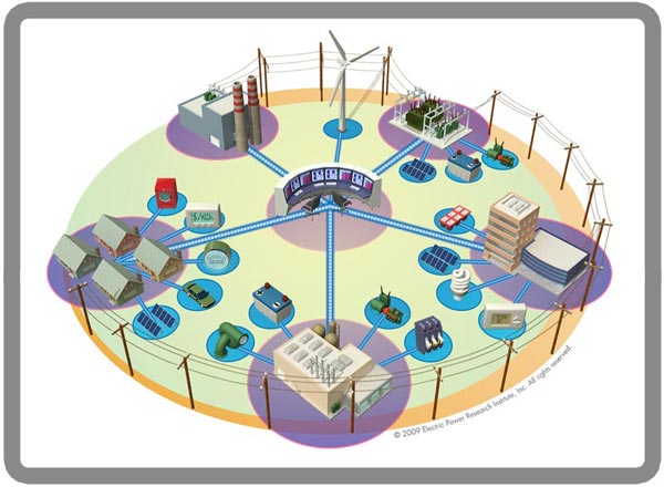
Smart grid
The principal case studies that will drive the development of the new framework consider CAS of socio-technical nature. The first is based on scalability analysis and capacity planning for smart urban transportation systems. Such systems are being adopted in many European cities to reduce CO2 emissions and pollutants and encourage green means of transportation. The main issues are ensuring that there is sufficient capacity within the system to avoid traffic congestion and traffic diversion, and investigation of the effect on users of adaptive, spatially dependent incentives. The second case study considers smart grid applications. In particular, the development of a general modelling and analysis framework will be driven by a number of problems regarding the modelling, prediction and control of such smart grids.
The QUANTICOL project is part of the EU FP7 FET Proactive Initiative on Fundamentals of Collective Adaptive Systems (FOCAS). The QUANTICOL consortium is composed of five partners:
• The University of Edinburgh, Edinburgh, U.K.
• The National Research Council of Italy, ISTI, Pisa, Italy
• Ludwig-Maximilians Univerity (LMU) Muenchen, Munich, Germany
• Ecole Polytechnique Federale de Lausanne, Lausanne, Switzerland
• IMT Institute for Advanced Studies, Lucca, Italy
![]()
![]()
![]()
![]()
![]()
Further information on the project can be found at: http://www.quanticol.eu.
(1) Susan Shaheen and Stacey Guzman (Fall 2011), "Worldwide Bikesharing". Access Magazine No. 39. University of California Transportation Center. Retrieved 2013-05-14 via wikipedia.
A network-aware extension of the pi-calculus
A key aspect of modern network architectures is the possibility of manipulating the network structure at run-time. For instance, in Software Defined Networks [1] switches are instructed to install or remove forwarding rules at run-time by a controller machine; in IaaS Cloud Computing systems new nodes and links, equipped with a specific amount of storage, bandwidth, access rights..., can be allocated whenever needed.
Traditional process calculi, such as the pi-calculus, CCS and others, seem inadequate to describe these kinds of systems, because they abstract away from network details. In this post we give an overview of Network Conscious pi-calculus (NCPi) [1,2], an extension of the pi-calculus with a natural notion of network. Following [2], we will first present a core version of NCPi, closer to the pi-calculus: we will recall the basic primitives of the pi-calculus and compare them with those of NCPi. Finally, we will present the "full-fledged" calculus.
Base calculus
The pi-calculus models communication over channels. These are represented as pure names, that are entities characterized only by their identity. The novelty w.r.t. CCS is that communicated data are channels themselves, so processes can increase their communication capabilities during computation. The basic operations are output and input along channels: ab.p is a process that can send b along a and continue as p, and a(x).q can receive at a some datum that will replace x in the continuation q.
NCPi models communication over a network. There are two kinds of names: sites, atomic names of the form a representing network nodes, and links, structured names of the form lab, representing a link with name l from a to b. In addition to the same input and output primitives as the pi-calculus, NCPi also has a primitive to activate a link: lab.p is a process that can provide a transportation service over lab to the environment and continue as p.
Both calculi have operators for executing two processes p and q in parallel, written p | q, and in a non-deterministic fashion, written p + q. The parallel execution may give rise to synchronizations, when the involved processes exchange messages. The synchronization mechanism is one major difference between the pi-calculus and NCPi. Both scenarios are exemplified in the following figures, where each process is depicted as a square with tentacles to its free names (only the relevant names are shown, which we assume to occur also in the subprocesses).
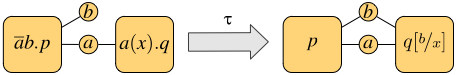
Synchronization in the pi-calculus
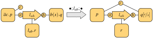
Synchronization in NCPi
The first figure shows the synchronization of the pi-calculus processes ab.p | a(x).q on the shared channel a: this gives rise to the observation tau and results in p and q sharing the channel b. In general, the pi-calculus only allows communication on shared channels, whereas NCPi is able to model remote communications. In fact, the second figure shows two processes that do not share output and input sites, but there is a process executing in parallel that provides a link between them, thus enabling the communication. The resulting observation is the link traversed by the datum. In general, a single communication may use a chain of links of arbitrary length.
NCP inherits the mechanism for creating and communicating new resources from the pi-calculus: fresh, unguessable sites and links are declared via the restriction operator (x)p, which binds x in p; communication of bound names enlarges their scope to the receiving process, which can use such names from then on. This is the mechanism that captures mobility.
Concurrent calculus
The calculus presented so far has an interleaving semantics, meaning that the behavior of parallel processes is given by their interleaved execution. This implicitly assumes the existence of a central arbiter who decides in which order resources should be accessed. However, such assumption can be considered inadequate for distributed systems with partially asynchronous behavior. We propose a version of NCPi which is closer to "real-life" networks. Its main features are:
- the output operator is of the form abc.p, modeling the emission of a packet from a with destination b and payload c.
- the semantics is concurrent, in the sense that many transmissions can be observed at the same time.
Concurrency in the semantics allows the associated behavioral equivalence to distinguish a parallel process from its interleaving counterpart (technically speaking, this avoids the usual counterexample where ab.a'(x) + a'(x).ab cannot simulate ab | a'(x) whenever a is identified with a', because the two processes are not equivalent in the first place). Indeed, it can be shown that such equivalence is preserved by all NCPi operators.
An example of parallel execution is depicted in the following figure.
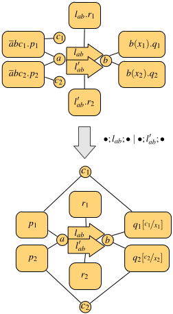
The top process has two links between a and b (for instance, one could be wired and the other one wireless). This enables the two processes on the left to transmit their data, both from a and addressed to b, at the same time. In fact, the resulting observation is made of two communications, each using one of the links from a to b, and both input variables are instantiated with actual values in the continuation (the bottom process).
[1] U. Montanari and M. Sammartino. Network conscious -calculus: A concurrent semantics. Electr. Notes Theor. Comput. Sci., 286:291–306, 2012. Available at http://www.di.unipi.it/ sammarti/papers/mfps28.pdf.
[2] U. Montanari and M. Sammartino. A network-conscious pi-calculus and its coalgebraic semantics. Theor. Comput. Sci. To Appear.
Analysing collective decision-making in swarm robotics
[Mieke Massink (ISTI) -- Joint work with Manuele Brambilla (ULB), Diego Latella (ISTI), Mauro Birattari (ULB) and Marco Dorigo (ULB)]
Analysing large and complex swarm robotics systems using physics-based simulations or directly with robots is often difficult and time consuming. For this reason, a common way to study these systems is by using abstract models. Models allow the developer to abstract from the complexity of a system and its implementation details and focus on the aspects that are relevant for the analysis.
An interesting problem in swarm robotics is how one can instruct robots in a swarm to make collective and optimal decisions. A further problem is then to find out whether a proposed strategy for decision making is indeed working as expected. The difficulties are caused by the fact that each robot in the swarm is on one hand operating independently from the others and on the other hand also cooperating with them and implicitly interacting with the environment creating feedback loops. Such feedback loops are known to be the cause of interesting phenomena such as that of emergent behaviour in the overall system that may sometimes be a desired effect as in the case of collective decision making.
Let's have a look at a concrete example and consider a swarm of robots that need to carry objects from a start area to a goal area. To carry an object, three robots are needed that work as a team. The start and the goal areas are connected by two paths: a short path and a twice as long path. The robots have to collectively identify and choose the shortest path. They do so by a voting process based on the majority rule [1] by the members of each team. Each robot has a preferred path. When a group is formed in the start area (Figure 1(a)), a vote takes place and the group chooses the path that is preferred by the majority of the robots it is composed of (Figure 1(b)). The chosen path also becomes the new preferred path for all the robots composing the group (Figure 1(e)). For example, if two robots prefer the short path and one robot prefers the long path, the short path is chosen for the next run and the robot that preferred the long path changes its preference to the short path. Note that the voting process takes place only in the start area and no other event can change the preference of the robots. Figure 1 shows a schema of the scenario. Initially half of the swarm prefers the short path and the other half the long one.
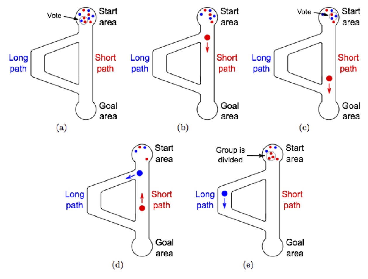
Fig. 1: Scenario
Since the robots taking the short path spend less time out of the start area than the robots taking the long path, their participation in the vote is, on average, more frequently establishing a positive feedback on the preference to vote for the short path. This results over time in the formation of more teams preferring the short path.
Recently, high-level modelling languages have been developed with which collective behaviour can be modelled using a population-oriented view-point. One of these languages is Bio-PEPA developed by Hillston et al. It is a variant of stochastic process algebra and therefore has important and useful properties such as compositionality: the overall system can be built from smaller basic components. But at least as important, different mathematical models can be derived from a Bio-PEPA specification that can be used in particular to analyse systems with a very large number of components applying analysis techniques such as stochastic simulation, statistical model checking and fluid flow analysis (see Fig. 2). The latter is a method that approximates, in a deterministic way, via differential equations, the change over time of the number of objects that are in a particular state. In our case for example the number of robots that prefer the short path.
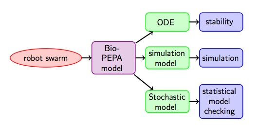
Fig. 2: Bio-PEPA analysis
This combination of a high-level language and sophisticated scalable analysis techniques makes it possible to analyse also swarms of large dimensions in an efficient way.
The idea of statistical model checking is to generate random executions of the system model and check whether they satisfy a particular property of interest (see Fig. 3). Statistical methods are then applied on the outcomes of those checks.
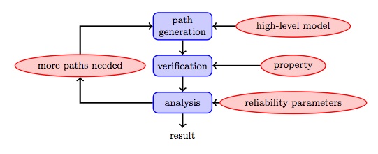
Fig. 3: Statistical Model-checking
For example, we can then automatically check what is the probability that the swarm reaches a decision and, if so, what is the probability that it is the desired decision. In Fig. 4 below the probability of convergence on the shortest path is shown for different average numbers of active teams k (and thus different numbers of robots that are in the start area at any time). For a swarm of 32 robots and with one path twice as long as the other the best probability is reached when there are on average about eight teams active. The results obtained with statistical model checking are comparable with those obtained via more common swarm robotics analysis methods such as physics-based simulation, but require much less time to be performed.
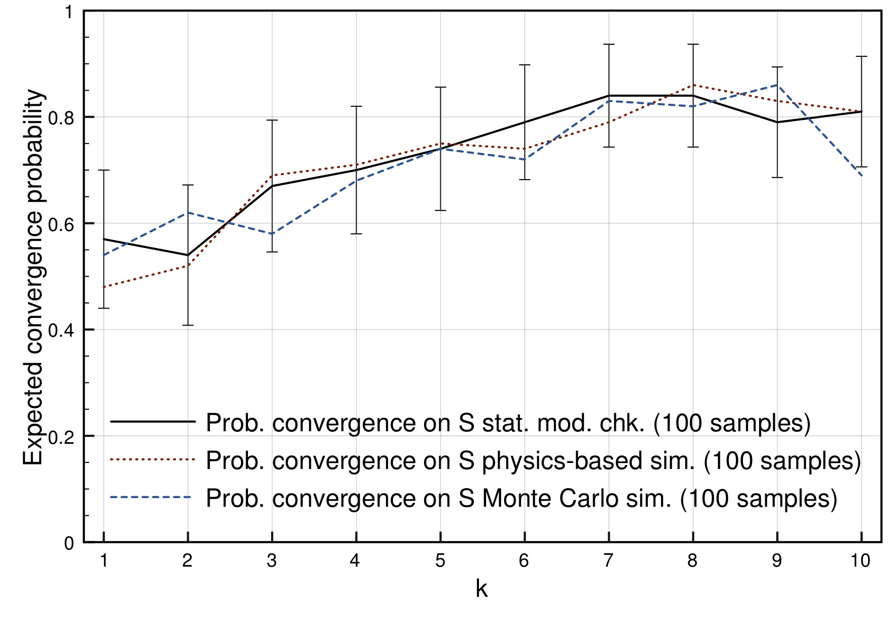
Fig. 4: Probability of convergence
What is even more of interest is that starting from a high-level language as Bio-PEPA it is easy to check what happens with the system under different circumstances. For example, what would happen if in the beginning the preferences for the different paths were not equally distributed among the robots in the start area. Or what would happen if most of the time almost all robots are away from the start area and the composition of teams could get easily biased or vary a lot due to the small number of robots from which a team would be selected. Or what would happen if some percentage of the robots would refuse to adjust their preference to comply with the majority.

Fig. 5: ODE solution
Fluid flow analysis of the same model may provide a computationally efficient way to get insight in the average behaviour of the swarm for very large populations. In Fig. 5 we see results for a swarm composed of 32,000 robots, all initially in the start area and then, when time passes many robots in the swarm leave this area and after a short while robots in favour of the short path S are increasingly dominating the population. The figure shows that the results of stochastic simulation (G1) of the whole system and the fluid (ODE) analysis are showing good correspondence, but the latter results are much faster to obtain and are insensitive to the actual size of the population.
A further research challenge will focus on analysing the effectiveness of decision strategies that can dynamically adapt to changing circumstances such as new shorter paths being created or optimal paths getting inaccessible.
References for further reading:
[1] M. A. Montes de Oca, E. Ferrante, A. Scheidler, C. Pinciroli, M. Birattari, and M. Dorigo. Majority-rule opinion dynamics with differential latency:
A mechanism for self-organized collective decision-making. Swarm Intelligence, 5(3-4):305-327, 2011.
[2] M. Massink, M. Brambilla, D. Latella, M. Dorigo, and M. Birattari. Analysing
robot swarm decision-making with Bio-PEPA. In Swarm Intelligence,
volume 7461 of Lecture Notes in Computer Science, pages 25-36. Springer,
Heidelberg, 2012.
[3] M. Massink, M. Brambilla, D. Latella, M. Dorigo, and M. Birattari. On the use of Bio-PEPA for Modelling and Analysing Collective Behaviours in Swarm Robotics. Swarm Intelligence, April 2013.
The Need of Rigorous Design of Ensembles
The increasing immersion and interaction of computing systems in both physical systems and societal systems, inevitably poses the problem of the nature of computing and its relationship to other scientific disciplines. What is the very nature of computing? How the interplay between different types of systems (physical, computing, biological) can be understood and mastered? To what extent can multi-disciplinary system-centric approaches contribute to a cross-fertilization of other disciplines?
Computing is a scientific discipline in its own right with its own concepts and paradigms. It deals with problems related to the representation, transformation and transmission of information. Information is an entity distinct from matter and energy. It is a resource that can be stored, transformed, transmitted and consumed. It is immaterial but needs media for its representation by using languages characterized by their syntax and semantics
Computing is not merely a branch of mathematics. Just as any other scientific discipline, it seeks validation of its theories on mathematical grounds. But mainly, and most importantly, it develops specific theory intended to explain and predict properties of systems that can be tested experimentally.
The advent of embedded systems brings computing closer to physics. Linking physical systems and computing systems requires a better understanding of differences and points of contact between them. Is it possible to define models of computation encompassing quantities such as physical time, physical memory and energy? Significant differences exist in the approaches and paradigms adopted by the two disciplines.
Physics is based on continuous mathematics while computing is rooted in discrete non-invertible mathematics. Physics studies a given “reality” and tries to discover laws governing physical phenomena while computing systems are human artifacts. Its laws are declarative by their nature. Physical systems are specified by differential equations involving relations between physical quantities. The essence of many physical phenomena can be captured by simple linear laws. They are, to a large extent, deterministic and predictable. Synthesis is the dominant paradigm in physical systems engineering. We know how to build artifacts meeting given requirements (e.g. bridges or circuits), by solving equations describing their behavior. By contrast, state equations of very simple computing systems, such as an RS flip-flop, do not admit linear representations in any finite field. Computing systems are described in executable formalisms such as programs and machines. Their behavior is intrinsically non-deterministic. Non-decidability of their essential properties implies poor predictability.
Computing enriches our knowledge with theory and models enabling a deeper understanding of discrete dynamic systems. It proposes a constructive and operational view of the world which complements the classic declarative approach adopted by physics.
Living organisms intimately combine interacting physical and computational phenomena that have a deep impact on their development and evolution. They share several characteristics with computing systems such as the use of memory, the distinction between hardware and software, and the use of languages. However, some essential differences exist. Computation in living organisms is robust, has built-in mechanisms for adaptivity and, most importantly, it allows the emergence of abstractions and concepts. We believe that these differences delimit a gap that is hard to be filled by actual computing systems.
The Design of Trustworthy Ensembles
The need for rigorous design is sometimes directly or indirectly questioned by developers of large-scale ensembles. These are systems of overwhelming complexity. They consist of an immense number of interconnected components and are built incrementally in an ad hoc manner. Their behavior can be studied only empirically by testing and through controlled experiments. The key issue is to determine tradeoffs between performance and cost by iterative tuning of parameters. Currently, a good deal of research on cloud-based or web-based systems privileges an analytic approach that aims to find laws that generate or explain observed phenomena rather than to investigate design principles for achieving a desired behavior. It is reported in [1] that “On line companies […] don’t anguish over how to design their Web sites. Instead they conduct controlled experiments by showing different versions to different groups of users until they have iterated to an optimal solution”.
This trend calls for two remarks.
- In contrast to physical sciences, computing is predominantly synthetic. Its main goal is to develop theory, methods and tools for building trustworthy and optimized computing systems. Considering the cyber-universe as a “given reality” driven by its own laws and privileging analytic approaches for their discovery and study, is epistemologically absurd and can have only limited scientific impact. The physical world is the result of a long and well-orchestrated evolution. It is governed by simple laws. To quote Einstein, “the most incomprehensible thing about the world is that it is at all comprehensible”. The trajectory of a projectile under gravity is a parabola which is a very simple and easy to understand law. There is nothing similar about programs or computing systems.
- Ad hoc and experimental approaches can be useful only for optimization purposes. Trustworthiness is a qualitative property and by its nature cannot be achieved by the fine tuning of parameters. Small changes can have a dramatic impact on safety and security properties.
We need theoretical frameworks that are expressive, make use of a minimal set of high level concepts and primitives for system description and that are amenable to formalization and analysis. Is it possible to find a mathematically elegant and still practicable theoretical framework for ensembles? We cannot expect to have theoretical settings as beautiful and as powerful as those for physical systems. One more profound reason is that computing systems are human artifacts while the physical systems are the result of a very long evolution.
In contrast to physical sciences that focus mainly on the discovery of laws, computing should focus mainly on theory for correct-by-construction and predictable system design. Design is central to the discipline. Awareness of its centrality is a chance to reinvigorate research, and build new scientific foundations matching the needs for increasing system integration and new applications.
There already exists a large body of correct-by-construction results such as algorithms, architectures and protocols. Their application allows correctness for (almost) free. How can global properties of ensembles be effectively inferred from the properties of their constituents? This remains an old open problem that urgently needs answers. Failure to bring satisfactory solutions will be a limiting factor for ensemble integration. It would also mean that computing is definitely relegated to second-class status with respect to other scientific disciplines.
J. Sifakis.
[1] Timo Hannay “The Controlled Experiment” in John Brockman “This will make you smarter”, Happer Perennial.
Which is the best robotic scenario to test our ensembles?
This question is a recurrent one in many projects dealing with mobile robotics and there is no largely recognized benchmarking scenario. Often the validation scenarios are adapted to the approach of the project, allowing to better show the performances of the proposed approach, of course. In ASCENS we have a different goal: we need a scenario where the various parameters can be modulated, where we can check a global approach and meet several challenges: modeling of complex environments or tasks, optimization, need for adaptation, fault tolerance, task allocation, constrains satisfaction, etc. Moreover the scenario has to be implemented both in simulation and on real robots.
Although not recognized as a benchmarking scenario in the whole mobile robotics community, "foraging" represent a class of tasks that is often used, especially in bio-inspired robotics. This task already includes coverage of an area, transportation and storage. These subtasks allow already dealing with task allocation and resources optimization challenges, for instance. Despite all this, we still found this task too simple and decided to add one interesting constraint: an external toxic source, potentially damaging the robots themselves. The final scenario looks very much like a "search and rescue" scenario, described in the following illustration:
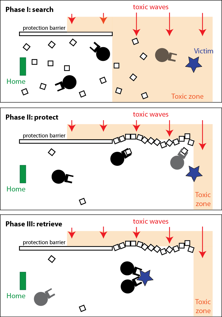
Illustration of the rescuing scenario in three phases.
In this scenario we have a home and a victim to rescue in a toxic environment. The home is in a safe zone protected from the toxic waves by a protection wall. The victim is in a zone exposed to the toxic waves. Within the environment there are construction blocks that can be used to build protection walls. The goal is to bring the victim to the home. We can split the whole mission in three phases: search, protect and retrieve.
This scenario is very interesting because it allows exploring, among others:
- Various types of tasks such as exploration, target location, transport of building blocks, construction and collective transport of large objects.
- Sequential as well as parallel actions. Robots can search and in parallel protect, or run these two phases in a sequential way.
- Task allocation, as robots could have different tasks.
- Optimization of resources, as robots have limited resources and could be damaged by the toxic waves.
- Bio-inspired as well as classical AI approaches.
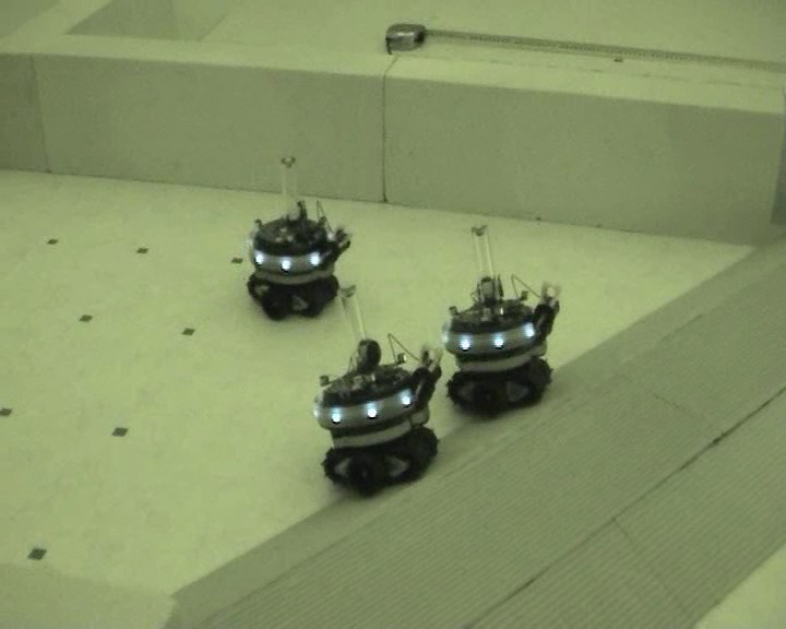
- Simulated and real implementations, as all elements of the scenario can be implemented using our marXbot robots. The toxic waves can be implemented using a lateral light source, colored or modulated.
All these aspects can be pushed to the highest complexity, or reduced to permit simple solutions, depending on the focus of the research. We believe that we have here all the components to generate a set of compatible scenarios that can, combined, address a class of real-world applications.
Francesco Mondada and Michael Bonani
Engineering Distributed Adaptive Systems using Components
Traditional software engineering methodologies together with related programming paradigms have long been guiding the procedure of building software systems through the requirements and design phase to testing and deployment. In particular, engineering paradigms based on the notion of components have gained a lot of popularity as they support separation of concerns - extremely valuable when dealing with systems of high complexity.
It seems, though, that these traditional methodologies and paradigms are not sufficient when exploited in the domain of continuously changing, massively distributed and dynamic systems, such as the ones we explore in the ASCENS project. These systems need to adjust to changes in their architecture and environment seamlessly or, even better, acknowledge the absence of absolute certainty over their (constantly changing) architecture and environment. An appealing research direction seems to be the decomposition of such systems into components able to operate upon temporary and volatile information in an autonomous and self-adaptive fashion. From the software engineering perspective, two main challenges arise:
- What are the correct low-level abstractions (models, respective paradigms) that will allow for separation of concerns?
- How can we devise a systematic approach for designing such systems, exploiting the above abstractions?
In response, we propose the DEECo component model (stands for Dependable Emergent Ensembles of Components). The goal of the component model is allow for designing systems consisting of autonomous, self-aware, and adaptable components, which are implicitly organized in groups called ensembles. To this end, we propose a slightly different way of perceiving a component; i.e., as a self-aware unit of computation, relying solely on its local data that are subject to modification during the execution time. The whole communication process relies on automatic data exchange among components, entirely externalized and automated within the runtime. This way, the components have to be programmed as autonomous units, without relying on whether/how the distributed communication is performed, which makes them very robust and suitable for rapidly-changing environments.
Main Concepts
DEECo is centered around two first-class concepts: component and ensemble. These two concepts closely reflect fundamentals of the SCEL specification language. In fact, DEECo is meant to be a component model that provides software engineering constructs for SCEL concepts. Consequently, the behavior of a system of DEECo components and ensembles can be described in SCEL in a straightforward way. The two first-class DEECo concepts are in detail elaborated below:
Component
A component is an autonomous unit of deployment and computation. Similar to SCEL, it consists of:
- Knowledge
- Processes
Knowledge contains all the data and functions of the component. It is a hierarchical data structure mapping identifiers to (potentially structured) values. Values are either statically typed data or functions. Thus DEECo employs statically-typed data and functions as first-class entities. We assume pure functions without side effects.
Processes, each of them being essentially a “thread”, operate upon the knowledge of the component. A process employs a function from the knowledge of the component to perform its task. As any function is assumed to have no side effects, a process defines mapping of the knowledge to the actual parameters of the employed function (input knowledge), as well as mapping of the return value back to the knowledge (output knowledge). A process can be either periodic or triggered. A process can be triggered when its input knowledge changes or when a given condition on the component’s knowledge (guard) is satisfied.
Ensemble
Ensembles determine composition of components. Composition is flat, expressed implicitly via a dynamic involvement in an ensemble. An ensemble consists of multiple member components and a single coordinator component. The only allowed form of communication among components is communication between a member and the coordinator in an ensemble. This allows the coordinator to apply various communication policies.
Thus, an ensemble is described pair-wise, defining the couples coordinator – member. An ensemble definition consists of:
- Required interface of the coordinator and a member
- Membership function
- Mapping function
Interface is a structural prescription for a view on a part of the component’s knowledge. An interface is associated with a component’s knowledge by means of duck typing; i.e., if a component’s knowledge has the structure prescribed by an interface, then the component reifies the interface. In other words, an interface represents a partial view on the knowledge.
Membership function declaratively expresses the condition, under which two components represent the pair coordinator-member of an ensemble. The condition is defined upon the knowledge of the components. In the situation where a component satisfies the membership functions of multiple ensembles, we envision a mechanism for deciding whether all or only a subset of the candidate ensembles should be applied. Currently, we employ a simple mechanism of a partial order over the ensembles for this purpose (the “maximal” ensemble of the comparable ones is selected, the ensembles which are incomparable are applied simultaneously).
Mapping function expresses the implicit distributed communication between the coordinator and a member. It ensures that the relevant knowledge changes in one component get propagated to the other component. However, it is up to the framework when/how often the mapping function is invoked. Note that (except for component processes) the single-writer rule applies also to mapping function. We assume a separate mapping for each of the directions coordinator-member, member-coordinator.
The important idea is that the components do not know anything about ensembles (including their membership in an ensemble). They only work with their own local knowledge, which gets implicitly updated whenever the component is part of a suitable ensemble.
Example
To illustrate the above-described concepts, we’ll give an example from the Science Cloud case-study. In this scenario, several interconnected, heterogeneous network nodes (execution nodes, storage nodes) run a cloud platform, on which 3rd-party services are being executed. Moreover, the nodes can dynamically enter/leave the network. Provided an external mechanism for migrating a service from one (execution) node to another, the goal is to “cooperatively distribute the load of the overloaded (execution) nodes in the network.”
Solution in a Nutshell
Before describing the solution in DEECo concepts, we will give an outline of the final result. Basically, for the purpose of this illustration, we consider a simple solution, where each of the nodes tracks its own load and if the load is higher than a fixed threshold, it selects a set of services to be migrated out. Consequently, all the nodes with low-enough load (determined by another fixed threshold) are given information about the services selected for migration, pick some of them and migrate them in using the external migration mechanism.
The challenge here is to decide which of the nodes the service information should be given to and when, since the nodes join and leave the network dynamically. In DEECo, this is solved by describing such a node interaction declaratively, so that it can be carried out in an automated way by the runtime framework when appropriate.
Realization in DEECo
Specifically, we first identify the components in the system and their internal knowledge. In this example, the components will be all the different nodes (execution/storage nodes) running the cloud platform (Figure 1). The inherent knowledge of execution nodes is their current load, information about running services, etc. We expect an execution node component to have a process, which determines the services to be migrated in case of overload. Similarly, the inherent knowledge of the storage nodes is their current capacity, filesystem, etc.
Figure 1. Components representing the cloud nodes and their inherent knowledge.
The second step is to define the actual component interaction and exchange of their knowledge. In this example, only the transfer of the information about services to be migrated from the overloaded nodes to the idle nodes is defined. The interaction is captured in a form of an ensemble definition (Figure 2), thus representing a “template” for interaction. Here, the coordinator, as well as the members, has to be an execution node providing the load and serviceInfo knowledge entries. Having such nodes, whenever the (potential) coordinator has the load above 90% and a (potential) member has the load below 20% (i.e., the membership function returns true), the ensemble is established and its mapping function is executed (possibly in a periodic manner). The mapping function in this case ensures exchanging the information about the services to be migrated from the coordinator to the members of the ensemble.

Figure 2. Definition of an ensemble that ensures exchange of the services to be migrated.
When applied to the current state of the components in the system, an ensemble - established according to the above-described definition - ensures an exchange of the service-to-be-migrated information among exactly the pairs of components meeting the membership condition of the ensemble (Figure 3).
Figure 3. Application of the ensemble definition from Figure 2 to the components from Figure 1.
According to the exchange of service information, the member nodes then individually perform service migration via the external (i.e., outside of DEECo) migration mechanism.
Current Implementation & Future Vision
As for implementation, we work on a prototype based on distributed tuple spaces and implemented in Java. The sources, as well as documentation and examples, can be found at https://github.com/d3scomp/JDEECo.
We envision that the component model outlined here will serve as the basis for a design methodology that will exploit the presented abstractions and help in building long-lasting systems of service-components and service-component ensembles.
Is your software adaptive?
As business processes and software architectures have started to extend beyond the boundaries of corporate systems through the Internet, computing systems have been facing a complete new set of expectations as well as market opportunities. Not only there has been an increasing complexity to be met for guaranteeing that the offered networks and services are trustworthy, but the need of designing and implementing open, loosely coupled services has come together with rapidly changing requirements to be met, with severe time-to-market constraints to be met and with unpredictable service compositions to be anticipated. In principle, autonomic systems are the best answer to these challenges, because they are capable to self-adapt to changing scenarios. In practice, there is no common agreement in the literature on what makes a system be adaptive, so that autonomic systems can be engineered under completely different and possibly conflicting strategies and operating guidelines.
Self-adaptive systems have been widely studied in several disciplines ranging from Biology to Economy and Sociology and there it is widely accepted that a system is self-adaptive if it can modify its behaviour as a reaction to a change in its context (e.g., the environment, the knowledge accumulated). But the problem with such definition emerges during the translation to the Computer Science setting, because it becomes too ambiguous to be helpful in discriminating adaptive systems from non-adaptive ones. In fact, most programs can change behaviour (as they can execute conditional statements, handle exceptions, etc.) as a reaction to a change in their context (as they can input data, modify parameters, etc.). And then, must an adaptive system always be capable to react to any change? Or does it suffice that it may adapt to some changes? Typically the behaviour is changed to improve some measure of performance or degree of satisfaction, but there can be no warranty about that, so what if the opposite happens? Does a system that decreases its performance deserve to be called adaptive?
As an example, consider the scenario of a speaker at a meeting that wants to connect her notebook to the beamer for given her presentation. The software of the notebook and of the beamer has been designed separately, without knowing which kind of beamer (resp. notebook) will be connected to, an agreement must be found for choosing the resolution at which the beamer will work and it is maybe the case that the resolution of the screen of the laptop will change as a consequence. Given these premises, one is lead to conclude that beamer and the notebook are adaptive systems. But what if we are told that the beamer is controlled by a loop that tries to synch with the notebook, starting from the highest resolution to lower ones until a common resolution is found? Isn't this just a default behaviour? Would you still call the beamer adaptive? And the notebook?
As a more interesting example, take the swarms of robots studied in the ASCENS case studies and one of the many challenging adaptation scenarios, like the hill crossing one, where the robots must self-assemble
if they encounter a hill to steep to climb alone. Looking at one of the video demo is impressive: the robots try and fail several time until they finally succeed (or maybe some robots is left alone behind). There is little doubt in calling the software of the robots (self-)adaptive. Still, a closer look at the so-called basic self-assembling strategy they run reveal a finite state machine controlling the adaptation strategy, not much different than a few conditional statement in a program in the end.
Puzzled by the above examples and many similar ones, we have come to the conclusion that the main problem with definition given above is that it relies on a black box view of the system, where an observer tries to classify the system without looking at the software it runs. This is reasonable in many other fields where adaptive systems have been studied, like Biology, because we cannot have a direct look at the "software" and we need to guess it. But the assumption is no longer valid in software systems, especially when the designer perspective is taken, not the user one.
The ambiguity becomes less striking when we take a white boxview of the system. In fact, many architectural approaches to autonomic systems take radically different guidelines on the way they can be structured or composed and on the way they operate. However, in most cases, such approaches are prescriptive: they take an underlying principle and explain how to build autonomic system according to that principle. For example, in the FORMS approach (FOrmal Reference Model for Self-adaptation) reflection is taken as a necessary criterion for any self-adaptive system: roughly, it must be capable to represent and manipulate a meta-level description of itself / of its behaviour. In the MAPE-K approach a self-adaptive system is made of a component implementing the application logic, equipped with a control loop that Monitors the execution through sensors, Analyses the collected data, Plans an adaptation strategy, and finally Executes the adaptation of the managed component through effectors; all the phases of the control loop access a shared Knowledge repository. While FORMS and MAPE-K are not necessarily conflicting, they suggest diverging architectures: in the case of MAPE-K, a strictly hierarchical structure is recommended, where the application logic of one layer implements the adaptation logic of the layer below and the two are to be kept well separated; in the case of FORMS it is favoured a mixture of application logic and adaptation logic by the use of reflection at the level of the application logic.
In a recent work we have proposed an architecture-agnostic, conceptual framework for adaptation, where the white box view of the system is essential. The crux of the framework is that the decision of whether a system is adaptive or not is a relative matter, not an absolute one.
According to a traditional paradigm, a program governing the behaviour of a component is made of control and data : these are two conceptual ingredients that in presence of sufficient resources (like computing power, memory or sensors) determine the behaviour of the component. In order to introduce adaptivity in this framework, we require to make explicit the fact that the behaviour of a component depends on some well identified control data, without being prescriptive on the way it is marked as such. Then: we define adaptation just as the run-time modification of the control data; we say that a system is adaptive if its control data are modified at run-time, at least in some of its executions; and we say that a system is self-adaptive if it is able to modify its own control data at run-time.
Ideally, a sensible collection of control data should be chosen to enforce a separation of concerns, allowing to distinguish neatly, if possible, the activities relevant for adaptation (those that affect the control data) from those relevant for the application logic only (that should not modify the control data). Then, any computational model or programming language can be used to implement an adaptive system, just by identifying the part of the data governing the behaviour. Consequently, the nature of control data can greatly vary depending on the degree of adaptivity of the system and on the computational formalisms used to implement it. Examples of control data include configuration variables, rules (in rule-based programming), contexts (in context-oriented programming), interactions (in connector-centred approaches), policies (in policy-driven languages), aspects (in aspect-oriented languages), monads and effects (in functional languages), and even entire programs (in models of computation exhibiting higher-order or reflective features).
So, coming back to the question posed in the title of this post, if you need to decide if you software system is adaptive or not, you need to name your control data first, then the rest will follow.
Challenges of Engineer Autonomic Behaviors
A well recognized research challenge for future large-scale pervasive computing scenarios relates to the need of enforcing autonomic, self-managing and self-adaptive, behaviour, both at the level of the infrastructure and at that of its services.
Indeed, the increasing decentralization and dynamics of the current and emerging ICT scenarios (a variety of highly-distributed devices of an ephemeral and/or mobile nature, with users and developers capable of injecting new components and services at any time) make it impossible for developers and system managers to stay in the control loop and directly intervene in the system for configuration and maintenance activities (e.g., for configuring or personalizing new distributed devices or services, for fixing problems in existing devices and services, or for optimizing resource exploitation).
Accordingly, in the past few years, a large number of research proposals have been made, at both the infrastructural and service levels, to promote autonomic and adaptive behaviour in pervasive computing systems. However, in our opinion, most of the current proposals suffer from several limitations when dived in future scenarios.
First, a number of approaches propose “add-ons” to be integrated in existing frameworks as, e.g., in the case of those autonomic computing approach “à la IBM”, suggesting coupling sophisticated control loops to existing systems to support self-management. The result is often in an increased complexity of current frameworks, which definitely does not suit the characteristics and the need for lightness of pervasive scenarios.
Second, a number of other proposals suggest relying on light-weight and fully decentralized approaches, typically inspired by natural phenomena of self-organization and self-adaptation. However, most of these exploit the natural inspiration only for the implementation of specific algorithmic solutions or for realizing specific distributed services, either at the infrastructural or at the user level, rather than for attacking the issue of autonomic self-adaptation in a comprehensive way.
Third, and although an increasing number of researchers focuses on the social aspects of pervasive computing and on the provisioning of innovative social services, they do not properly account for the social level as an indistinguishable dimension of the overall pervasive computing fabric. That is, they do not account for the fact that users, other than simply consumers or producers of services, are de facto devices of the overall infrastructure, and contribute to it via human sensing, actuating, and computing capabilities, other than via an inherent strive for adaptation.
Based on the above considerations, our belief is that – rather than looking for one-of solutions to specific adaptation problems from specific limited viewpoints – there is need to deeply rethink the modelling and architecting of modern pervasive systems. As challenging as this can be, one should try to account in a foundational and holistic way for the overall complex needs of adaptation and autonomic behaviour of future pervasive computing systems. The final goal should be that of making such systems inherently capable of autonomic self-management and adaptation at the collective level, and having the distinction between infrastructural, services, and social levels, blur or vanish completely.
The achievement of the outlined broad goal calls for facing a number of specific challenging research issues, necessary to compose the global picture. These may include, among the others:
- Supporting Comprehensive Self-awareness. While the need for situation-awareness is already a recognized issue in pervasive computing, future scenarios will require autonomous adaptation activities to be driven by more comprehensive levels of awareness than traditionally enforced in context-aware computing models, where it is typically up to each component to access and digest the information it needs to take adaptation decisions. Such awareness models should encompass situations occurring at the many different levels of the system, as well as the strict locality of components, and be eventually able to provide components of the pervasive computing infrastructure with expressive and compact representations of complex multi-faceted situations, so as to effectively drive each and every activity of the components in a collectively coordinated way.
- Reconciling Top-Down vs Bottom Up Approaches. Along with the traditional “top-down” approaches to the engineering of pervasive computing systems, in which specific functionalities or behaviour are achieved by explicit design, “bottom-up” approaches are being proposed and adopted too (as we have already anticipated), to achieve functionalities via spontaneous self-organization, as it happens in natural systems. Most likely, both approaches will coexist in future pervasive computing scenarios, the former applied to the engineering of specific local functionalities, the latter applied to the engineering of large-scale behaviours (or simply emerge as a natural collective phenomena of the system). Thus, there will be need to understand the trade-offs between the power of top-down adaptation and bottom-up one, also by studying how the two approaches can coexist and possibly conflict in future systems, and possibly contributing in smoothing the tension between the two.
- Enforcing Decentralized Control. In large-scale systems, we should never forget that the existence and exploitation of phenomena of collective adaptation must necessarily come along with models and tools making it possible to control “by design” the overall behaviour of the pervasive systems and its sub-parts. Clearly, due to the inherent decentralization of the systems, such control tools too should make it possibly to direct the behaviours of the system in a decentralized way, and should be coupled by means to “measure” such behaviours in order to understand if the control is effective. The issue of defining sound measures for future pervasive computing scenarios can define in itself a challenging research area, given the size of the target scenario and the many – and often quite ill-defined – purposes it has to concurrently serve.
The need for laying out brand new foundations for the modelling and architecting of autonomic and self-adaptive pervasive computing systems, opens up a large number of fascinating and challenging research questions. In the ASCENS project, we are trying to understand how it is possible to identify a sound set of self-aware adaptation patterns for ensemble, and how such patterns can be used for engineering both top-down and bottom-up adaptation schemes, other than for enforcing in a decentralized way control over the global behaviour of ensembles.
In any case, the short list of challenges that we have provided above and that we are currently tackling in ASCENS is far from being exhaustive. For instance, it does not account for the many inter-disciplinary issues that the understanding of large-scale socio-technical organisms (as future pervasive computing systems will be) and their collective adaptive behaviours involve , calling from exploiting the modern lessons of applied psychology, sociology, social anthropology, and macro-economy, other than those of systemic biology, ecology and complexity science. Plenty of room for additional projects to complement ASCENS!
Formal Methods for Computer System Engineering
[This post is the continuation of "What can Formal Methods do?", which I posted to this blog on Jan. 31, 2012. In that post I tried to motivate the need of Formal Methods (FMs) in Computer System Engineering (SE). In the present post I briefly sketch some of the basic concepts and notions in the area of FMs for concurrent systems]
Let me start by recalling the quotation I made in my previous post: “All engineering disciplines make progress by employing mathematically based notations and methods.” [Jon00]. C. Jones continues as follows: “Research on `formal methods' follows this model and attempts to identify and develop mathematical approaches that can contribute to the task of creating computer systems”. This statement is complemented by what W. Thomas writes in the same book, i.e. FMs “Attempt to provide the (software) engineer with concepts and techniques as thinking tools, which are clean, adequate, and convenient, to support him (or her) in describing, reasoning about, and constructing complex software and hardware systems” [Tho00].
In a nutshell, we can say the FMs for Computer System Engineering (SE) find their roots in Theoretical Computer Science (TCS) and in Mathematical Logics (ML) but they differ from both TCS and ML in their primary goal, which is pragmatic rather than foundational with emphasis on construction, automatic (often `push button’) software tool support, rather then on fundamental questions like computability of completeness (in the technical sense) of theories. In the following I’ll show a simple example of logic/mathematics notions and structures used in FMs for SE. For space reasons I’ll consider only the case of abstractions for distributed, actually concurrent, systems, i.e. systems composed of (very) many components, where each component (usually) performs (very) simple tasks (often sequential), but the interaction among components is usually complex, difficult to understand, non-deterministic, and subtle (due to race conditions, synchronization issues, dead-/live-locks, etc.). This choice does not mean (by no means!) that non-concurrent systems are easy to design or that the theory behind such systems is not interesting. Extremely important foundational work has been produced in the area of sequential computing, including the basics of computability theory, of operational and denotational semantics, formal program analysis and transformation, etc. The choice is mainly due to reasonable space limitations, to the focus of ASCENS as well as personal taste and competence.
Most mathematical structures used for modelling concurrent systems are variants of Labelled Transition Systems (LTSs). Often, such models are syntactically represented as terms of suitable Process Algebras (PAs, well ... PAs are, as the words themselves should suggest, much more than just languages for specifying models!). LTSs are state-transition structures, i.e. structures in which the behaviour of a system is modelled by means of a set of (global) states, which the system can be in, and a set of transitions, which describe how a system can move from which state to which one. What a state is depends on what the designer wants to model: states are not necessarily associated to specific information `per se’. This is a point where system designer ingenuity is crucial. A state could be associated to a specific set of voltages at the components of an electrical circuit, in which case a transition would correspond to a possible change in such values. I guess we can agree that such a modelling choice would probably bring to models with huge numbers of states and transitions! More realistically one could think of associating a different state to each specific set of values of variables and execution points of the software components of a distributed system at a given point in time, in which case a transition would correspond to the execution of a command. But a state could also correspond to a certain position of the parts of a robot that are relevant for a certain application, in which case transitions would model possible changes of position. At an even more abstract level of modelling, a state could simply represent whether a given shared resource is free or not, and a transition would model granting or refusing a request of usage of that resource. Regardless of the specific interpretation we assign to states and transitions, a state-transition structure is a mathematical structure as follows: (S, -->) where S is a non-empty set of states (usually finite or denumerable) and --> is a binary relation on S. It is often useful to associate labels to transitions, denoting specific actions of our system, so that a typical definition of a LTS is a triple (S, L, -->), where L is a non-empty transition label set and --> is a relation over S x L x S; again, notice that typically, no particular assumption needs to be made on the elements of L, their specific interpretation being left to the designer of the specific model; in some cases, instead, it might be more convenient do fix a specific structure of labels.
We can use graphical notations as well:
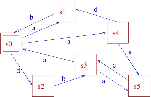
From the initial state s0, by executing action a, the system can get to state s1 or s4 (yes, some systems can be non-deterministic... ), while the execution of action d brings the system to state s2, and so on. You will also easily understand that the information captured by the above picture could very well be described textually, as follows:
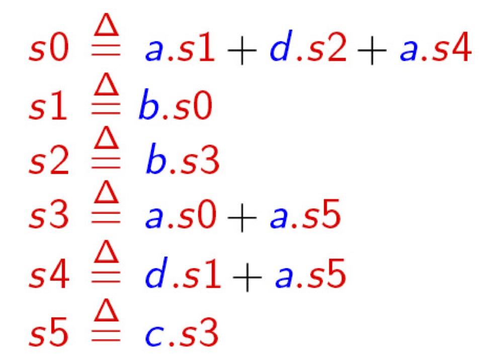 where the notation x.P specifies that a transition labelled by x brings the system to (the) state (specified by) P, and an expression like P1 + P2 specifies a state that may behave like (specified by) P1 or (specified by) P2, so that it should now be easy to infer that the behaviour specified above for our system when being in state, say, s0 is indeed that prescribed by the LTS in the picture, and so on. In some cases, one might find it useful to label states, instead of transitions; the resulting structures, known as Kripke Structures [after the famous logician], form the basis for the semantics of modal logics, which temporal logics are a special case of and represent one of the most successful tools for the formal specification of system requirements. Of course, we sometimes find it useful to have both state and transition labels. As the above example might have suggested, one can model more and more complex behaviours by means of composing simpler ones, using operators like . and +. In fact, many more operators are commonly used, including parallel composition ones, by means of which one can put different LTSs together and study the overall behaviour when they execute “in parallel”. So, the game is again to have (1) a set of basic components and (2) ways for composing them. In fact, what I’ve been briefly introducing with the above example is the notion of process algebra (PA), where we have a set of process terms and operators for composing them, with a formal definition of both the syntax of the relevant language, built out of such basic components and operators, and of its semantics, which relates language terms to LTSs. For the sake of simplicity, I refrained from elaborating here on the mathematics of syntax and semantics definition; the interested reader is referred to the literature.
There are a lot a mathematical results behind the name PA. For instance, appropriate process algebraic relations and in particular pre-orders and equivalences have been discovered, which allow us to compare process terms w.r.t. their behaviour and, e.g., to replace a process in a model with an equivalent (but maybe cheaper to implement) one, still keeping the behaviour of the overall model unchanged (do you remember the example of the resistors R1 and R2 which, when composed in a certain way can replace a third resistor, R, thanks to a mathematical relation between the three resistors and the specific composition pattern? ... Well, we are now doing something similar, but with computer system models!!). Furthermore, in many cases, those equivalences have a textual representation, in the form of general laws, exactly as it happens in elementary algebra (thus the name of process algebra). For instance, for any processes P1, P2, P3, it holds P1 + P2 = P2 + P1 and P1 + (P2+ P3) = (P1 + P2) + P3. This means that system models expressed in PA can be manipulated, sometimes mechanically/automatically, for discovering possible design bugs (e.g. the fact that a system, after a certain behaviour hangs up, i.e. is equivalent to the zero process nil, famous because it never performs any action ...), or for simplifying designs, etc. etc.
Furthermore, a formal link can be established between system designs expressed, for instance, as PA terms and system requirements, expressed, e.g. in temporal logics, as we mentioned before. For instance, with reference to the LTS of our example above, a sentence like "In all possible runs [of a system modelled by such an LTS] whenever the system is in state s0, it will eventually reach state s4", can be formally expressed in temporal logic (although, by the way, it does not hold in our example, since any system modelled by the above LTS may keep cycling forever as follows: s0,s2, s3, s0,s2, s3, s0,s2, s3, s0,s2, s3, ....). The link between the requirement specifications and the model of a system can be implemented into software tools (typically known as model-checkers) which automatically check whether a system model satisfies a given requirement, and, if not, even yield you back a counter-example.
PA, and in general LTS based techniques, have also a strong link with standard techniques for quantitative analysis of systems, e.g. performance. This can be expressed by means of enriching PA languages with probabilistic information so that they can describe performance models, like Continuous Time Markov Chains (CTMCs), without loosing their nice compositionality features, and even serve as a formal backbone for studying fluid limit properties of system models, by mean of sophisticated PA interpretations based ordinary differential equations. These, so called Stochastic PA, are equipped with more sophisticated logics for requirements specification, which are usually obtained as appropriate extensions of temporal logics, like the Continuous Stochastic Logic (CSL), which allows us to express requirements like , e.g.,: "The probability is larger than 0.97 that a swarm of robots will reach a given target by 4 minutes". Suitable tools for automatic stochastic model-checking are available which check whether a given stochastic model, possibly expressed as a stochastic PA term, satisfies a CSL---or some other stochastic logic---formula. Finally, models written using stochastic PAs can easily be simulated using stochastic simulation techniques, or, when the models would be too huge to be simulated, the relevant results can be approximated using fluid flow, ODE based, techniques.
I’ll refrain from discussing all this now here, and I refer the interested reader to the relevant literature in the areas of concurrency theory. The above was an attempt to show that there exists indeed basic math for the design of complex computer systems; and of course there exists much more than I could mention here, which is really a fragment of the overall body of FMs. There are some people that, at this point, are still suspicious about the real “practical usefulness” of FMs and thus they are sometimes surprised by the fact that research effort and funding is devoted to the study of mathematical foundations and FMs for computer system design. Would they be as well surprised by the fact that quite some math, and related research and development, has been involved in the centuries, and is still involved, in the design of buildings, bridges, ships or aircrafts? I think they should instead be surprised by the fact that still, too often, engineers do not use FMs in SE. I would be very much surprised, and scared, if I knew that a building, a bridge, a ship, an aircraft, or a complex critical software system was not designed and implemented using the support of sound and appropriate math! And if some people are still missing some success stories on the development and use of FMs, maybe it might help them knowing that current model-checking technologies can deal with LTSs with trillions of states, and in some cases with number of states of the order of 10 power 10.000 [CAS09], and that FMs have been successfully applied to critical space applications, like the Cassini probe system (see, e.g. http://spinroot.com/spin/whatispin.html), the Mars Exploration Rovers (see the Jan. 2004 issue of COMPUTER), the Deep Space. Nomad 1 system for Antartica exploration, or the design of the Rotterdam Storm Surge Barrier which protects The Netherlands from high water and is fully automated (no man in the loop, from weather forecast to closing the barrier!), just to mention the most spectacular systems which could have not been designed without the support of FMs,and related tools, in SE. To the above, one should then add the more routine-like use of FMs in the railway sector, among others.
And then ... looking for exciting use of FMs in autonomic service component ensembles? Stay connected with the ASCENS Project web site!
[CAS09] E. Clarke, E. Emerson, and J. Sifakis. Model Checking: Algorithmic Verification and Debugging. Turing Lecture. Communications of the ACM, Vol. 52, n. 11, November 2009, pages 75—84
[Jon00] C. Jones. Thinking Tools for the Future of Computing Science. In R. Wilhelm, editor. Informatics 10 Years Back 10 Years Ahead, volume 2000 of Lectures Notes in Computer Science. Springer-Verlag, 2000. pp 112-130
[Tho00] W. Thomas. Logic for Computer Science: The Engineering Challenge. In R. Wilhelm, editor. Informatics 10 Years Back 10 Years Ahead, volume 2000 of Lectures Notes in Computer Science. Springer-Verlag, 2000. pp 257—267.
What can Formal Methods do?
In a post of F. Tiezzi to this blog, titled “Robot Swarms – What can Formal Methods do?" it has been shown that Formal Methods (FMs) can support the development of models of real (robotics) systems and that such models can be used for system simulation. It has also been (correctly!) argued that such simulation offers many advantages, especially when compared with experimentation on the real system, e.g. in terms of cost. A possible objection to Francesco’s point could be: couldn’t simulation be performed as well using models built without the use of formal modelling languages and supporting theories? In the end, this is what computer professionals have been doing for decades . . . In other words, Francesco deliberately avoided addressing the issue ‘per se’ of the role of FMs in Computer System Engineering (SE), including the engineering of complex systems of autonomic service component ensembles.
In this post I’ll try instead to focus on this very issue. The reason why I decided to do so is that my personal experience induces me to think that the role of FMs in SE is still not fully appreciated in the Computer Science (CS) community, not even in the more intellectually sophisticated part thereof, namely in the CS research community. So, I think that a few considerations on this subject might help the reader understanding also why a great deal of ASCENS effort is devoted to the development of formal modelling and analysis languages and techniques. Of course, I have to apologize with all colleagues in the area of FMs, and in particular with ASCENS friends, for inaccuracies, and incomplete or obvious statements which unavoidably will pop up in my post; on the other hand, being this the public ASCENS blog I ask knowledgeable people to tolerate my superficiality, if this can help a broader community getting a chance to appreciate the role of, and the motivations for FMs. And, ultimately, also their role in ASCENS.
My first and, I’d say major, observation is that this lack of appreciation for FMs seems to be a peculiarity of people’s attitude towards SE, not at all experienced when considering other branches of engineering. Let me start by quoting C. Jones [Jon00]: “All engineering disciplines make progress by employing mathematically based notations and methods.” Notice that the above consideration applies to all engineering disciplines, and it explicitly refers to notations and methods that are mathematically based. Is this true?
Let us consider civil engineering. In this case, graphical notations, among others, are widely used, and this goes on now for quite a long time (see the figure below [MaJ06]):
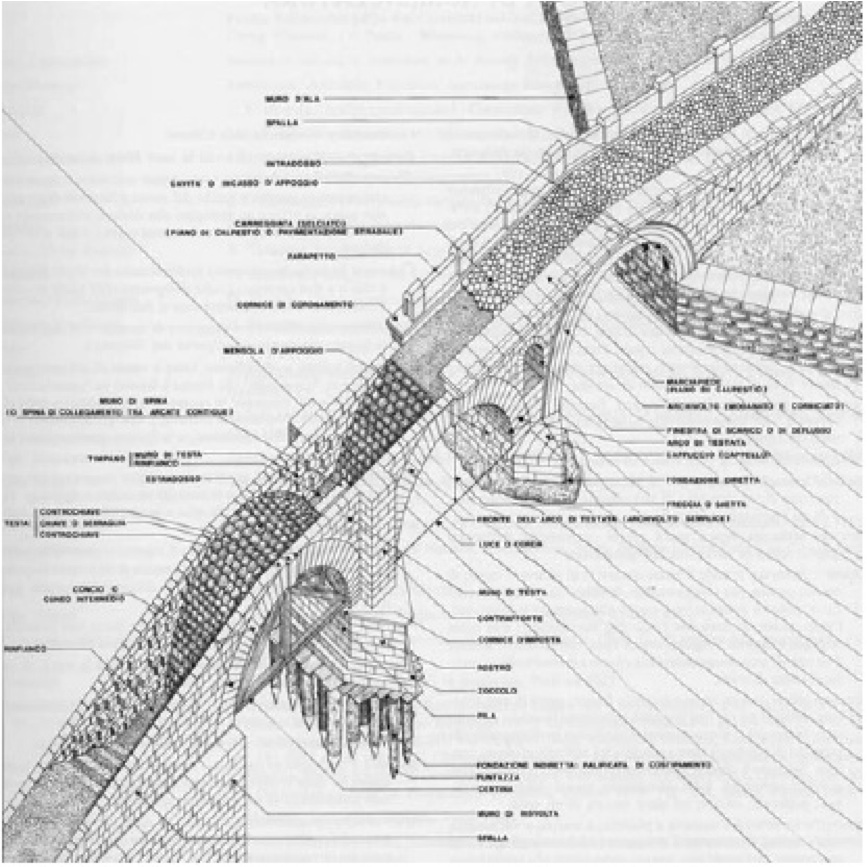
Although the result of using such graphical notations can be quite evocative, and may bear some artistic value, it is worth noting that technical drawing is regulated by rather strict rules. Such regulations are often internationally standardized and amazingly detailed (I still remember that when I was an undergraduate student, we were thought, at a technical drawing course, that when we draw a certain kind of arrows, the width of the tip should be in a fixed relationship with its length---1/3, to be precise, if I remember well!---in order for the arrow to be a “correct” one). Furthermore, we were thought specific techniques for constructing, or better, (almost) mechanically generating, “sections” of objects. Well … essentially, we were thought rigorous, sometimes formal, rules for drawing models of the artefacts we were designing, be them bridges or taps. To a certain extent, these rules were a rigorous definition of the syntax to be used for creating our models. On the other hand, the sectioning/projecting techniques were based on formal rules of mechanical manipulation of the drawings, . . . a, maybe rudimentary, form of model analysis based on formal semantics. Furthermore, in most cases, such drawings were decorated with numbers which could be used in mathematical formulas in close relation with (parts of) the drawings, or derivable from them (think, for instance, at the calculation of the max load which can safely cross a bridge, starting from the sizes, materials, and geometric relationships of the relevant components of the bridge, using the laws of statics).
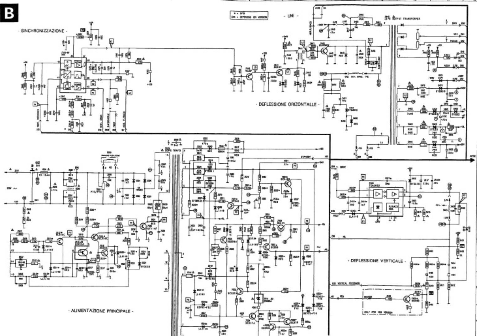
Another example of the close relationship between design notations and maths in the tradition of engineering is the design of electrical circuits. Below there is a typical (although dated!) example thereof, related to a commercial device (copyright PHILIPS):
You can see several instances of different kinds of components, connected in certain ways and with annotations, typically referring to (physical) quantities related to electricity. I want to elaborate a little bit more on electrical circuits and maths. To that purpose, let's use a simpler schema, which we all have probably got acquainted with at high school, the so-called RLC circuit.
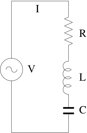 We immediately note that there are some basic components (for resistors, inductances, capacitors, etc.), possibly with some quantities associated with them, and standardized systematic ways of composing them (e.g. in series, in parallel, in series-parallel, etc.). Again, although the above graphic descriptions are quite evocative of the physical objects they represent, we can use them for reasoning about our designs in rather abstract and often mechanical ways, with the help of some math, and without necessarily having to experiment repeatedly with physical realizations of our circuits. For instance, as you will remember, by using Kirchhoff laws, we can predict that the resistance offered by the circuit below at its terminals is R=R1*R2/(R1+R2).
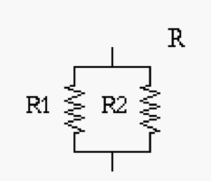
This formal, mathematical, relationship between R, R1, R2 and the associated composition diagram allows us to replace, in any circuit, e.g. the RLC one above, a resistor of a given resistance R, say 8 Ohm, with the parallel composition of two resistors R1, R2, of, say, 16 Ohm. Notice that we can make those manipulations directly on the graphical schema, even mechanically, provided the above equality is not violated. On the other hand, the above equality comes from specific laws of physics, which are, in turn, expressed as math formulas. Although we have been using a graphical notation for circuits, I’m sure you will understand that we could describe our systems using textual notations instead, based on operators, like, say, PARALLEL(x1,s2) or SERIES (x1,x2), etc.
A closer look at the RLC circuit, and some basic knowledge of physics, allow us to express the relationships between the components of the circuit and the physical quantities of interest, e.g. the current i and voltage v at the power unit terminals (PU), at any point in time, as follows:
![]()
The solution of the above equation gives a current that changes over time with a sine like shape
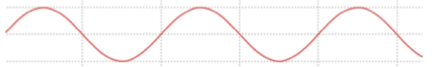
The frequency w of the sine is that specific of the PU. It is useful to study how the amplitude of the above signal, i.e. the (absolute) value of the peaks, changes with w. It can be shown that (for appropriate values of R, L, and C) as w increases from 0 the amplitude increases as well, reaches a max and then decreases again, as follows:
 The frequency corresponding the amplitude peak is the so-called resonance frequency (RF). Why is the RF so important? And, most of all, why am I bothering you with all these details? Both questions are easy to answer! The identification and study of RFs are of paramount importance in the design of systems that might be subject to oscillations (these include RLC circuits, but also bridges, ships, or aircrafts, for example); to be brief: devices and systems can be seriously damaged by too high oscillation amplitudes (bridges can crash, ships can sink or brake down...). For what concerns the second question, I used the above example for showing you that, starting from a diagram, sometimes called a blueprint, i.e. a formal syntactical description of a model of a system, and doing some manipulations of its semantics with the help of mathematics, we can characterize some peculiar features of the system we are designing. The document where the relevant peculiar features of a system are specified is the so-called technical specification, also called, in our, CS, domain, requirements specifications document. Needless to say, it is convenient that also such a document be as much rigorous as possible, even better, if it also includes some logic/mathematical formulas, as is the case for RLC systems (because this helps in having unambiguous specifications of the requirements). The process of relating a design model with the requirements specification can be seen as a process of abstraction and, of course, appropriate notions should be available also for checking that a design model satisfies a given requirement. But do we have to do all this by paper and pencil or only experimental testing? Fortunately not: we can play with software tools (see, e.g. http://ngsir.netfirms.com/englishhtm/RLC.htm), even forgetting, while designing and only to a certain extent, that behind all these activities there is a huge and solid body of mathematics supporting them, including Set Theory, Continuous Mathematics, Metric Spaces, Differential Calculus and Function Analysis, Linear Algebra, Differential Equations, just to mention a few ...
Summarizing: Civil, Naval, Nuclear, Electrical, Electronic (. . .) Engineers use notations for technical specifications (requirements specifications) as well as design specifications/models that
- are strongly based on mathematics (and physics),
- are compositional (at least in a broad sense),
- are characterized by great and flexible descriptive power,
- allow for the formal manipulation of their objects
- are heavily supported by computer (software) tools (e.g. for model analysis, including relating models to technical specs)
Society expects engineers to be aware of the underlying theories although not necessarily to be able to completely master them. I repeat it: a good, or even average, civil, electrical, etc. engineer, is socially not allowed to claim he can do without formal methods. And now: what about engineers designing complex, critical, computer/software systems? Although in the past there have been people, including respectable scientists, who have been arguing that SE is mainly a matter of art, or, at most of kraft-work, there is now some consensus, at least in the SE community itself, that it is a matter of engineering and so, as in any other branch of engineering, besides ingenuity and inspiration, there is need of systematic application of sound methodologies and techniques, with a solid mathematical basis.
But then, the question is what is the logics/mathematics basis of SE: what kind of mathematical objects, theories and techniques can best support the design activities typical of SE. I’ll touch upon these issues soon, in my next post.
[Jon00] C. Jones. Thinking Tools for the Future of Computing Science. In R. Wilhelm, editor. Informatics 10 Years Back 10 Years Ahead, volume 2000 of Lectures Notes in Computer Science. Springer-Verlag, 2000 112-130
[MaJ06] M. Mazzoleni, L. Jurina ``PONTI IN MURATURA: DIFETTI E PATOLOGIE'', CIAS 2006, Bolzano