Formal Methods for Computer System Engineering
[This post is the continuation of "What can Formal Methods do?", which I posted to this blog on Jan. 31, 2012. In that post I tried to motivate the need of Formal Methods (FMs) in Computer System Engineering (SE). In the present post I briefly sketch some of the basic concepts and notions in the area of FMs for concurrent systems]
Let me start by recalling the quotation I made in my previous post: “All engineering disciplines make progress by employing mathematically based notations and methods.” [Jon00]. C. Jones continues as follows: “Research on `formal methods' follows this model and attempts to identify and develop mathematical approaches that can contribute to the task of creating computer systems”. This statement is complemented by what W. Thomas writes in the same book, i.e. FMs “Attempt to provide the (software) engineer with concepts and techniques as thinking tools, which are clean, adequate, and convenient, to support him (or her) in describing, reasoning about, and constructing complex software and hardware systems” [Tho00].
In a nutshell, we can say the FMs for Computer System Engineering (SE) find their roots in Theoretical Computer Science (TCS) and in Mathematical Logics (ML) but they differ from both TCS and ML in their primary goal, which is pragmatic rather than foundational with emphasis on construction, automatic (often `push button’) software tool support, rather then on fundamental questions like computability of completeness (in the technical sense) of theories. In the following I’ll show a simple example of logic/mathematics notions and structures used in FMs for SE. For space reasons I’ll consider only the case of abstractions for distributed, actually concurrent, systems, i.e. systems composed of (very) many components, where each component (usually) performs (very) simple tasks (often sequential), but the interaction among components is usually complex, difficult to understand, non-deterministic, and subtle (due to race conditions, synchronization issues, dead-/live-locks, etc.). This choice does not mean (by no means!) that non-concurrent systems are easy to design or that the theory behind such systems is not interesting. Extremely important foundational work has been produced in the area of sequential computing, including the basics of computability theory, of operational and denotational semantics, formal program analysis and transformation, etc. The choice is mainly due to reasonable space limitations, to the focus of ASCENS as well as personal taste and competence.
Most mathematical structures used for modelling concurrent systems are variants of Labelled Transition Systems (LTSs). Often, such models are syntactically represented as terms of suitable Process Algebras (PAs, well ... PAs are, as the words themselves should suggest, much more than just languages for specifying models!). LTSs are state-transition structures, i.e. structures in which the behaviour of a system is modelled by means of a set of (global) states, which the system can be in, and a set of transitions, which describe how a system can move from which state to which one. What a state is depends on what the designer wants to model: states are not necessarily associated to specific information `per se’. This is a point where system designer ingenuity is crucial. A state could be associated to a specific set of voltages at the components of an electrical circuit, in which case a transition would correspond to a possible change in such values. I guess we can agree that such a modelling choice would probably bring to models with huge numbers of states and transitions! More realistically one could think of associating a different state to each specific set of values of variables and execution points of the software components of a distributed system at a given point in time, in which case a transition would correspond to the execution of a command. But a state could also correspond to a certain position of the parts of a robot that are relevant for a certain application, in which case transitions would model possible changes of position. At an even more abstract level of modelling, a state could simply represent whether a given shared resource is free or not, and a transition would model granting or refusing a request of usage of that resource. Regardless of the specific interpretation we assign to states and transitions, a state-transition structure is a mathematical structure as follows: (S, -->) where S is a non-empty set of states (usually finite or denumerable) and --> is a binary relation on S. It is often useful to associate labels to transitions, denoting specific actions of our system, so that a typical definition of a LTS is a triple (S, L, -->), where L is a non-empty transition label set and --> is a relation over S x L x S; again, notice that typically, no particular assumption needs to be made on the elements of L, their specific interpretation being left to the designer of the specific model; in some cases, instead, it might be more convenient do fix a specific structure of labels.
We can use graphical notations as well:
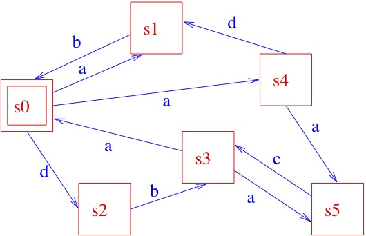
From the initial state s0, by executing action a, the system can get to state s1 or s4 (yes, some systems can be non-deterministic... ), while the execution of action d brings the system to state s2, and so on. You will also easily understand that the information captured by the above picture could very well be described textually, as follows:
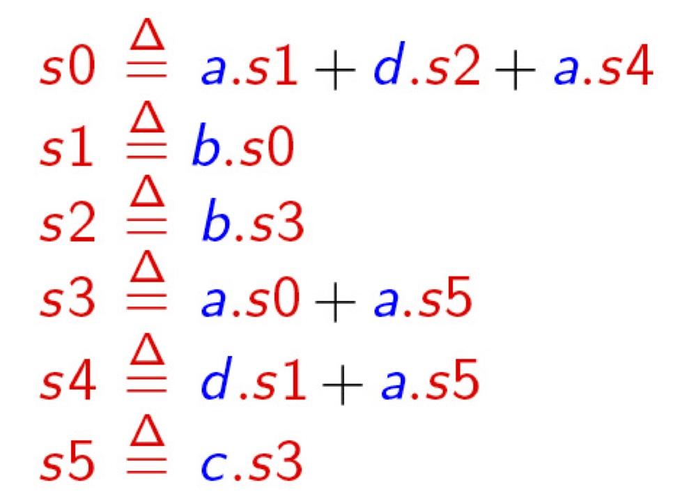 where the notation x.P specifies that a transition labelled by x brings the system to (the) state (specified by) P, and an expression like P1 + P2 specifies a state that may behave like (specified by) P1 or (specified by) P2, so that it should now be easy to infer that the behaviour specified above for our system when being in state, say, s0 is indeed that prescribed by the LTS in the picture, and so on. In some cases, one might find it useful to label states, instead of transitions; the resulting structures, known as Kripke Structures [after the famous logician], form the basis for the semantics of modal logics, which temporal logics are a special case of and represent one of the most successful tools for the formal specification of system requirements. Of course, we sometimes find it useful to have both state and transition labels. As the above example might have suggested, one can model more and more complex behaviours by means of composing simpler ones, using operators like . and +. In fact, many more operators are commonly used, including parallel composition ones, by means of which one can put different LTSs together and study the overall behaviour when they execute “in parallel”. So, the game is again to have (1) a set of basic components and (2) ways for composing them. In fact, what I’ve been briefly introducing with the above example is the notion of process algebra (PA), where we have a set of process terms and operators for composing them, with a formal definition of both the syntax of the relevant language, built out of such basic components and operators, and of its semantics, which relates language terms to LTSs. For the sake of simplicity, I refrained from elaborating here on the mathematics of syntax and semantics definition; the interested reader is referred to the literature.
There are a lot a mathematical results behind the name PA. For instance, appropriate process algebraic relations and in particular pre-orders and equivalences have been discovered, which allow us to compare process terms w.r.t. their behaviour and, e.g., to replace a process in a model with an equivalent (but maybe cheaper to implement) one, still keeping the behaviour of the overall model unchanged (do you remember the example of the resistors R1 and R2 which, when composed in a certain way can replace a third resistor, R, thanks to a mathematical relation between the three resistors and the specific composition pattern? ... Well, we are now doing something similar, but with computer system models!!). Furthermore, in many cases, those equivalences have a textual representation, in the form of general laws, exactly as it happens in elementary algebra (thus the name of process algebra). For instance, for any processes P1, P2, P3, it holds P1 + P2 = P2 + P1 and P1 + (P2+ P3) = (P1 + P2) + P3. This means that system models expressed in PA can be manipulated, sometimes mechanically/automatically, for discovering possible design bugs (e.g. the fact that a system, after a certain behaviour hangs up, i.e. is equivalent to the zero process nil, famous because it never performs any action ...), or for simplifying designs, etc. etc.
Furthermore, a formal link can be established between system designs expressed, for instance, as PA terms and system requirements, expressed, e.g. in temporal logics, as we mentioned before. For instance, with reference to the LTS of our example above, a sentence like "In all possible runs [of a system modelled by such an LTS] whenever the system is in state s0, it will eventually reach state s4", can be formally expressed in temporal logic (although, by the way, it does not hold in our example, since any system modelled by the above LTS may keep cycling forever as follows: s0,s2, s3, s0,s2, s3, s0,s2, s3, s0,s2, s3, ....). The link between the requirement specifications and the model of a system can be implemented into software tools (typically known as model-checkers) which automatically check whether a system model satisfies a given requirement, and, if not, even yield you back a counter-example.
PA, and in general LTS based techniques, have also a strong link with standard techniques for quantitative analysis of systems, e.g. performance. This can be expressed by means of enriching PA languages with probabilistic information so that they can describe performance models, like Continuous Time Markov Chains (CTMCs), without loosing their nice compositionality features, and even serve as a formal backbone for studying fluid limit properties of system models, by mean of sophisticated PA interpretations based ordinary differential equations. These, so called Stochastic PA, are equipped with more sophisticated logics for requirements specification, which are usually obtained as appropriate extensions of temporal logics, like the Continuous Stochastic Logic (CSL), which allows us to express requirements like , e.g.,: "The probability is larger than 0.97 that a swarm of robots will reach a given target by 4 minutes". Suitable tools for automatic stochastic model-checking are available which check whether a given stochastic model, possibly expressed as a stochastic PA term, satisfies a CSL---or some other stochastic logic---formula. Finally, models written using stochastic PAs can easily be simulated using stochastic simulation techniques, or, when the models would be too huge to be simulated, the relevant results can be approximated using fluid flow, ODE based, techniques.
I’ll refrain from discussing all this now here, and I refer the interested reader to the relevant literature in the areas of concurrency theory. The above was an attempt to show that there exists indeed basic math for the design of complex computer systems; and of course there exists much more than I could mention here, which is really a fragment of the overall body of FMs. There are some people that, at this point, are still suspicious about the real “practical usefulness” of FMs and thus they are sometimes surprised by the fact that research effort and funding is devoted to the study of mathematical foundations and FMs for computer system design. Would they be as well surprised by the fact that quite some math, and related research and development, has been involved in the centuries, and is still involved, in the design of buildings, bridges, ships or aircrafts? I think they should instead be surprised by the fact that still, too often, engineers do not use FMs in SE. I would be very much surprised, and scared, if I knew that a building, a bridge, a ship, an aircraft, or a complex critical software system was not designed and implemented using the support of sound and appropriate math! And if some people are still missing some success stories on the development and use of FMs, maybe it might help them knowing that current model-checking technologies can deal with LTSs with trillions of states, and in some cases with number of states of the order of 10 power 10.000 [CAS09], and that FMs have been successfully applied to critical space applications, like the Cassini probe system (see, e.g. http://spinroot.com/spin/whatispin.html), the Mars Exploration Rovers (see the Jan. 2004 issue of COMPUTER), the Deep Space. Nomad 1 system for Antartica exploration, or the design of the Rotterdam Storm Surge Barrier which protects The Netherlands from high water and is fully automated (no man in the loop, from weather forecast to closing the barrier!), just to mention the most spectacular systems which could have not been designed without the support of FMs,and related tools, in SE. To the above, one should then add the more routine-like use of FMs in the railway sector, among others.
And then ... looking for exciting use of FMs in autonomic service component ensembles? Stay connected with the ASCENS Project web site!
[CAS09] E. Clarke, E. Emerson, and J. Sifakis. Model Checking: Algorithmic Verification and Debugging. Turing Lecture. Communications of the ACM, Vol. 52, n. 11, November 2009, pages 75—84
[Jon00] C. Jones. Thinking Tools for the Future of Computing Science. In R. Wilhelm, editor. Informatics 10 Years Back 10 Years Ahead, volume 2000 of Lectures Notes in Computer Science. Springer-Verlag, 2000. pp 112-130
[Tho00] W. Thomas. Logic for Computer Science: The Engineering Challenge. In R. Wilhelm, editor. Informatics 10 Years Back 10 Years Ahead, volume 2000 of Lectures Notes in Computer Science. Springer-Verlag, 2000. pp 257—267.